Physically based rendering, or short PBR, is a collection of techniques that aims to create a graphical representation that is based on physics. There is no official guide to what encompasses "PBR" but there are defently some concepts that come to most peoples mind when talking about PBR. Physically based rendering is usually rooted in the rendering equation so lets start by talking about that.
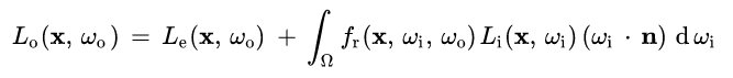
First of all, we will need to get acquainted with the rendering equation
It might look a bit complex at first glance, but its really not that complicated and you dont even need to understand integrals to grasp what we are going to do (the integral part will be irrelevant which will be explained going further into this article).
We will simplify the rendering equation until we end up with a special, restricted case of the rendering equation which is called the reflectance equation. To be able to drop the integral part we will make some further simplificaitons. We will use a simplified light source model, only focus on local illumination and we also wont have support for environment lighting.
The simplifed model we create will only support local illumination where as the rendering equation above can be used for Global Illumination - the key difference being that our local illumination model only depends on knowledge of distinct light sources and not other surfaces in the scene to determine the incoming light (in a global illumination model we would also like to take into account light bouncing off other surfaces in the scene). As we will see, this simplification is one of the reasons we can do without an integral - we can easily determine where all of our incoming lights are. Our light model also does'nt try to do any form of environment lighting, where it would be necessary to have some sort of a spherical or hemispherical function to account for the incoming light surrounding the fragment.
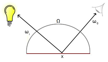
The rendering equation is based on a integral. This serves to consider any light coming in at a direction around the hemisphere surronding the point x. The picture bellow illustrates the concept and how we will simplify it so that we no longer need to evaluate an integral in our shader.
One way to implement the rendering equation with the integral approach would be to try to divided the hemisphere (Ω) into steps. A pseudo solution could look something like this:
int nrSteps  = 100;
float dW = 1.0f / nrSteps;

// X is the fragment position, Wo the direction from X to camera and N the surface normal
vec3 X    = ...;
vec3 Wo   = ...;
vec3 N    = ...;

float value = 0.0f;
for(int i = 0; i < nrSteps; i++)
{
    vec3 Wi = getIncomingLightDirection(i);
    value += Fr(X, Wi, Wo) * L(X, Wi) * dot(N, Wi) * dW;
}
This seems like quite a cumbersome way to approach it. Since we already know where the lights are, we can easily find the light direction ωi for all the types of lights we want to support (this article will cover a point light but the same would work for directional and spot lights as well).
What we do instead is that we will iterate over all lights in the scene and find ωi for that light. This eliminates the need to use an integral.
The next part that we want to do to simplify things for us is to substitute the Li(x,ωi) part of the equation. From the rendering equation, Li(x,ωi) is the light radiance coming from the hemisphere in and hitting position x. Since we know all the lights in our scene, we can subsitute this with the light radiance from our lights.
In a PBR approach, it is common to use more sophisticated light source descriptions. In our example, we will be using infinitesimals light sources. What that means is that we have taken a real world light source (for example a light bulb) and modelled it as an infinitely small point with just a 3D position from where the light is emitted. This way, all we need in order to describe how much light that will reach the fragment is a vector.
In a more complex light source model, the light can be seen as an area. This will in general result in more realistic looking results (especially for smooth surfaces) but does require us to take solid angles into account in the Li(x, ω) function.
In the image bellow, the left side shows the model we are using and the right side shows the concept of an area light.

Given our choice of light source model, we could calculate how much light is reaching x from a point light by calculating the attenuation. Here is an example of how we could calculate the radiance of a point light:
vec3 lightColor = vec3(1.0f, 1.0f, 1.0f); // White light
float lightIntensity = 40.0f; // light intensity
float distance = length(lightPos - fragPos);
float attenuation = 1.0f / distance * distance;
vec3 radiance = lightCol * lightIntensity * attenuation;
There is one more thing that we will be removing from our rendering equation and that is the support for emitted radiance. Our shader will not be dealing with surfaces that can emit light. Lets look at the equation again.
Le(x, ωo) - this part deals with emitted radiance. In our case, this will always evalute to zero. Hence, we can just forget about it.
Lets have a look at the rendering equation again with our simplifications in place:
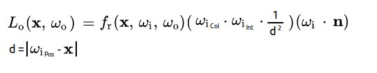
So we have dropped the Le(x, ωo) and replaced Li(x,ωi) with the radiance of a point light. We have also removed the integral and decided that we will instead iterate over all the light sources in the scene and sum up the result of the above equation. The last part of the equation, ωi * n, is just a dot product.
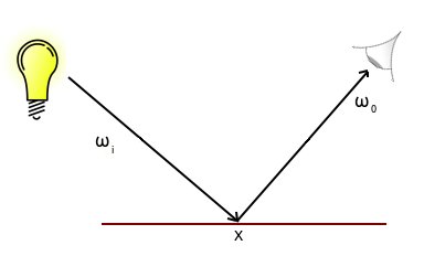
This equation is what our shader will be based on and the final color of the fragment is the result of the function denoted Lo. The output from Lo is the light reflected from a fragment x viewed from the angle ωo.
A pseudo code solution could look something like this:
/*
    W = vector with light information
    Wo = vector from fragment position to eye
    x = fragment position
    n = surface normal
*/

vec3 outCol = vec3(0.0f, 0.0f, 0.0f);

for(int i = 0; i < numLights; i++)
{
    float d = length(W[i].pos - x);
    float attenuation = 1.0f / d * d;
    float radiance = W[i].col * W[i].int * attenuation;

    // Assumes we are working with a point light here
    vec3 lightDirection = W[i].pos - x;
    outCol += Fr(x, lightDirection, Wo) * radiance * dot(lightDirection, n);
}

outCol = clamp(OutCol, 0, 1);
All that is left is to explore is the fr(x,ωi,ωo), the BRDF function, which is what we will focus on for the remainder of this article.
fr(x,ωi,ωo) is a Bidirectional reflectance distribution function (short BRDF), which is the heart of our lighting model. Using a description of the material the fragment is made of, the incoming light and the viewing angle of the fragment our BRDF will be able to produce the reflected color of the fragment visible from the camera.
Our BRDF will be able to output two types of surface response to the incoming light:
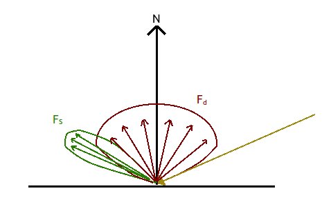
The image above illustrates the light response from a single incoming ray hitting the surface - the diffuse component being light scattered evenly outwards from the point the light hit and the specular component here as a lobe shape.
The complete surface response from our BRDF would be these two components put together. To make it easier to reason about them we will therefore describe the complete surface respones as f(x,ωi,ωo) = fd + fs
The diffuse component is based on Lambert's Cosine Law, which basically says that the more aligned the incoming light ray is with the surfaces normal, the greater the diffuse reflection will be.
This is not very different from the diffuse shading we did in Rendering (diffuse section) - we are still measuring the angle between the incoming light ray and the surface normal. But this happens in the form of a dot product in our simplified rendering equation, lets have a look at it again:
Here, we can see the last part - (ωi * n). This is the same as the cosine of the angle between ωi and n. fd, in our BRDF, will therefore instead be a constant:
fd = c / π
c in the equation above is the albedo color(we will go over what albedo means later on). The reason why we arrive at this factor is not trivial. But it comes down to the fact that light that is diffusely reflected should be equally reflected across a hemisphere surrounding the fragment that was lit by the incoming light. The amount of light that is evenly distributed across this hemisphere must not be more than what was reflected from the fragment. There is an excellent explanation of the details of this here which I could recommend.
The specular component is calculated as:
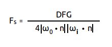
Where
Before we get into the the specular part, we need to explore microfacet theory. A BRDF based on the microfacet theory is good at generating realistic looking lighting, which is why it is a very popular approach and common when talking about PBR.
The basic idea is that all surfaces, when looked at under close inspection, consist of many very small facets. Each of these facets acts as a perfect specular reflector.
A clay pot, while having a pretty smooth surface to the naked eye will reveal quite a rough surface if you look at it closer. A smoother surface, like a polished metal will show much less jaggies when looking at the surface closer.


A rougher surface will tend to scatter the light more in a seemingly random way (left image bellow), while a smoother surface will produce a more uniform reflection (right image bellow.)


The Normal Distribution Functions (NDF) "job" is to estimate how the normals of the microfacets align with the halfway vector. This can be achieved by using a roughness factor to describe if the surface is either smooth or rough.
For a smooth surface, there will be a small area of the surface where many of the microfacets will align with the halfway vector, giving a bright, clear specular lobe. On a rougher surface, there will instead by many microfacets that somewhat align with the halfway vector, giving the surface a bigger but not quite as intense specular lobe.
The NDF determines the shape of the specular lobe, as well as how the borders of the specular lobe looks. This is illustrated in the example bellow, showing two isotropic NDFs. The top row is Beckmann - where the border of the specular lobe is clear. The bottom one shows Trowbridge-Reitz "GGX", which has more of a haze around the specular lobe. The roughness factor is lowest at the left and highest at the right.
 and Trowbridge-Reitz (bottom)")
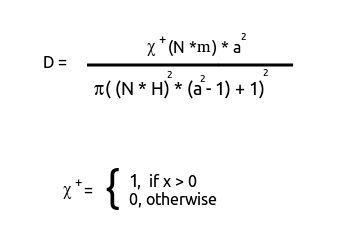
When modelling anisotropic materials, such as brushed metals, one needs to use an anisotropic NDF. Bellow is an example of an anisotropic NDF (from Disney). Here, the shape of the specular lobe is stretched out like a ring across the surface.

While there are many NDFs, the most common is probably the Trowbridge-Reitz GGX which is the one we will be using.
This is what the equation looks like
The first part of the equation, in the χ+ function, can be replaced with 1. The reason is that we assume that all the microsurface normals are facing outwards (which means that the dot product of N and m will always be > 0).
Bellow is the shader code for the NDF function
// H - halfway vector
// N - surface normal
//----------------------------------------------------------------------------
float DistributionGGX(vec3 N, vec3 H, float roughness)
{
    float a = roughness*roughness; // Disney’s style, a = Roughness * Rougness
    float a2 = a*a;
    float NdotH = clamp(dot(N, H), 0.0, 1.0);
    float NdotH2 = NdotH*NdotH;

    float nom   = a2;
    float denom = (NdotH2 * (a2 - 1.0) + 1.0);
    denom = PI * denom * denom;

    return nom / denom;
}
Geometric shadowing refers to the occlusion of visible microfacets as well as the shadowing of microfacets. We are once again back to the microfacet theory, which says that a surface that is flat to the naked eye is actually made up of many small microfacets. These microfacet will sometimes cast shadows onto other (visible) microfacets as well as occlude some microfacets. This can be seen in the image bellow
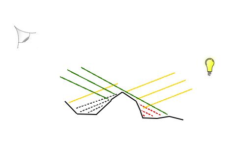
The yellow lines are incoming light, the green lines indicate fragments visible to the camera. The black doted lines on the left show the shadowing effect of the microfacets. The red dotted lines on the right show microfacets that are occluded by other microfacets.
There are BRDFs that also account for interreflection among the microfacets, but we will not venture into that in this section. Instead we will opt to settle for a joint masking-shadowing function, that is a geometric function that account for both occlusion and shadowing (but not interreflection).
Our G function will evaluate occlusion and shadowing separetly and then multiply the results together and that result is what we use for geometric shadowing. This is a common variant as proposed by Heitz("Understanding the Masking-Shadowing Function in Microfacet-Based BRDFs", section 6 "The Smith Joint Masking-Shadowing Function" page 44)
The G1 function can be varied, the one we will be using is the suggested by Walter et al. ("Microfacet Models for Refraction through Rough Surfaces", page 7)
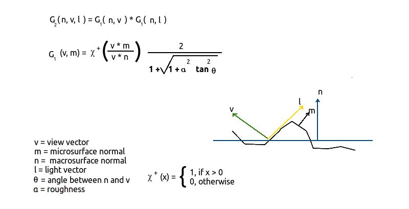
As can be seen in the picture above, we can calculate the shadowing and occlusion effect by the function denominated G2. It, in turn, uses the G1 function for both the shadowing and occlusion and then multiplies the results together. This is a simplification in that it assumes that occlusion and shadowing are uncorrelated events, in reality they are not and this casues this function to make the end result darker then it should be. It is, however, still very commonly used and will suffice for our purposes.
The first thing to notice in the G1 function is the value in the χ+ function. This will always evalute to 1 since we assume that both the macrosurface and microsurfaces are facing outwards.
Bellow is the fragment shader code
float G1_GGX(float Ndotv, float alphaG)
{
    return 2 / (1 + sqrt(1 + alphaG*alphaG * (1-Ndotv*Ndotv)/(Ndotv*Ndotv)));
}
//----------------------------------------------------------------------------
float GeometrySmith(vec3 N, vec3 V, vec3 L, float roughness)
{
    float NdotV = max(dot(N, V), 0.0);
    float NdotL = max(dot(N, L), 0.0);
    float GGXV = G1_GGX(NdotV, roughness);
    float GGXL = G1_GGX(NdotL, roughness);

    return GGXV * GGXL;
}
The fresnel equation is a way to describe the ratio of how much light is refracted and how much is reflected.
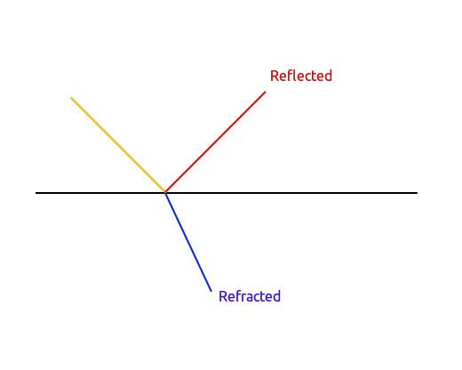
The image above illustrates a "surface interface" (shown by the black line in the picture) surronded by air. The yellow light is an incoming light ray and the red line is the light that bounces of it. The blue line is the light that is refracted into the surface. In our case, a "surface interface" is the triangles making up the visible meshes in our scene.
The phenomenon usually associated with Fresnel is the highlight that can be seen at grazing angles of an object.
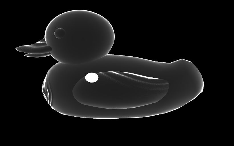
This can be seen in the picture above, the surfaces of the duck that face us straight on get almost no lighting but as the angle between the surface normal and our view approaches 90 degrees, the surface is intensely lit. This is the Fresnel effect (The white sphere is the light source).
There is one more important characteristic that we will model in our Fresnel function, and that is how conductors (metals) and dielectrics (example plastics) effect the reflected light. Conductors will tint the light, dielectrics do not alter the reflected light.
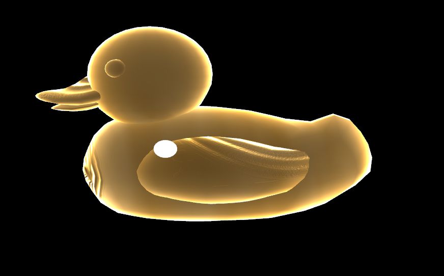
The image above is the same duck model but with a metal surface - the color of the light reflected is tinted by the material. The highlights at the grazing angles remain the same - as the angle between the surface and our view direction approaches 90 the reflected light will be white.
We will use the Schlick approximation of the Fresnel effect, which can be described as:
Our Fresnel function acts as an RGB interpolation from F0 to pure white. In order to support both dielectrics and metals (conductors), we will vary F0. If its a dielectric, F0 will be (0.04, 0.04, 0.04). If it is a metal, however, we will change F0 to the color of that material. This is what allows our lighting model to support tinting the reflected light color when we are dealing with a material that is a metal.
This is where we introduce the "metallic" component of a material. Just as we used a roughness component to control the specular lobe, we also have a "metallic" component which indicates how metallic the surface is. In reality, a material is either a metal or not - it can't be something in between. But to make it more convenient for artists to get the right look of the material (ex a mixed material) we can define a material as being somewhere inbetween. The metallic component is introduced the same as the roughness, a value from 0 - 1. We get our F0 value using linear interpolation as:
// Fresnel base reflectivity, dia-electric (plastic) has 0.04 IOR
vec3 F0 = vec3(0.04);
F0 = mix(F0, albedoColor, metallic);
If the metallic value is 0 - we will get a dielectric F0 = (0.04, 0.04, 0.04). If its more metallic, we interpolate from dielectric base reflectivity to the value stored in the albedo texture map. It is worht noting that this is a simplification of representing the Fresnel effect - but its quite a good one without introducing unreasonably complex or calculation heavy code.
Bellow is the fragment shader code of the Fresnel function:
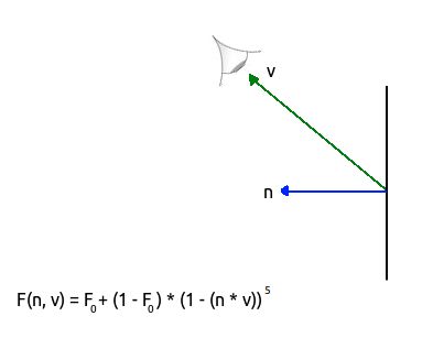
// cosTheta - dot product of halfway vector and the eye direction vector
// F0 - "Base" reflectivity
vec3 fresnelSchlick(float cosTheta, vec3 F0)
{
    return F0 + (1.0 - F0) * pow(1.0 - cosTheta, 5.0);
}
The last thing we need to get a beliveable look is to make sure our BRDF follows the rules of energy conservation: outgoing light energy should never exceed the incoming light. If it did, we would have surfaces that acts as surface emitters.
This can become especially troublesome in case where we add support for global illumination, the picture bellow illustrates the problem in the left image - extra emitted light has been bouncing around inside the sphere causing it to look like its glowing from inside (source Physically-Based Materials – Energy Conservation and Reciprocity)

In order to preserve energy conservation, we need a way to differ between light that has been absorbed into an object and light that has bounced (reflected) right off of it.
As you have just read the part about Fresnel, that might ring a bell. The Fresnel factor will give use the light which has bounced off the object to produce part of the specular lobe. This means that the energy part remaining for the diffuse part must be 1.0 - the Fresnel factor.
// kS is equal to Fresnel
vec3 kS = F;
// for energy conservation, the diffuse and specular light can't
// be above 1.0 (unless the surface emits light); to preserve this
// relationship the diffuse component (kD) should equal 1.0 - kS.
vec3 kD = vec3(1.0) - kS;
#version 330 core

// Input vertex data
layout(location = 0) in vec3 vertexPosition_modelspace;
layout(location = 1) in vec3 vertexNormal_modelspace;
layout(location = 2) in vec2 vertexUV;
layout(location = 3) in vec3 vertexTangent_modelspace;

out float gl_ClipDistance[1];

out vec3 position_worldspace;
out vec3 eyeDirection_tangentspace;
out vec3 lightDirection_tangentspace;
out vec2 UV;


uniform mat4 MVP; // ModelViewProjection
uniform mat4 V; // View
uniform mat4 M; // Model
uniform mat4 MV; // ModelView
uniform mat3 MV3By3; // ModelView Top left part only, leaving out translation as we are only using this matrix to operate on normals anyways
uniform mat4 NM; // Normal Matrix, the transpose inverse of the ModelView matrix
uniform vec3 lightPosition_worldspace;
uniform vec4 userClipPlane0; // user defined clip plane in view-space

void main()
{
	gl_Position =  MVP * vec4(vertexPosition_modelspace,1);

	// Calculate data needed for lighing in fragment shader
	vec3 vertexPosition_cameraspace = ( MV * vec4(vertexPosition_modelspace,1)).xyz;

	// Position of the vertex in worldspace
	position_worldspace = (M * vec4(vertexPosition_modelspace,1)).xyz;

	// Need homogenus space location for the clipping
	vec4 position_worldspaceVec4 = vec4(position_worldspace.x, position_worldspace.y, position_worldspace.z, 1);

	gl_ClipDistance[0] = dot(position_worldspaceVec4, userClipPlane0);

	vec3 cameraPosition = vec3(0,0,0); // OpenGLs camera position is always fixed at 0,0,0 looking down the negativite Z axis.
	vec3 eyeDirection_cameraspace = cameraPosition - vertexPosition_cameraspace;

	vec3 lightPosition_cameraspace = ( V * vec4(lightPosition_worldspace,1)).xyz;
	vec3 lightDirection_cameraspace = lightPosition_cameraspace - vertexPosition_cameraspace;

	vec3 vertexTangent_cameraspace 		= MV3By3 * normalize(vertexTangent_modelspace);
   	vec3 vertexNormal_cameraspace 		= MV3By3 * normalize(vertexNormal_modelspace);
	vec3 vertexBitangent_cameraspace	= MV3By3 * normalize(cross(vertexNormal_modelspace, vertexTangent_modelspace));

	// transpose in this case is the same as inverse, its just cheaper than doing inverse
	mat3 TBN = transpose(mat3(vertexTangent_cameraspace, vertexBitangent_cameraspace, vertexNormal_cameraspace));

 	lightDirection_tangentspace = TBN * lightDirection_cameraspace;
        eyeDirection_tangentspace =  TBN * eyeDirection_cameraspace;

	UV = vertexUV;
}
#version 330 core

// Interpolated values from the vertex shaders
in vec3 position_worldspace;
in vec3 eyeDirection_tangentspace;
in vec3 lightDirection_tangentspace;
in vec2 UV;

uniform sampler2D textureAlbedo;
uniform sampler2D textureNormal;
uniform sampler2D textureMetallic;
uniform sampler2D textureRoughness;
uniform sampler2D textureAO;

uniform vec3 lightPosition_worldspace;
uniform vec3 lightColor;
uniform float lightIntensity;

const float PI = 3.14159265359;

// Output data
//layout(location = 0) out vec3 color;
out vec3 color;

// cosTheta - dot product of [halfway vector] and the [eye direction vector]
// F0 - "Base" reflectivity
vec3 fresnelSchlick(float cosTheta, vec3 F0)
{
    return F0 + (1.0 - F0) * pow(1.0 - cosTheta, 5.0);
}
//----------------------------------------------------------------------------

// H - halfway vector
// N - surface normal
//----------------------------------------------------------------------------
float DistributionGGX(vec3 N, vec3 H, float roughness)
{
    float a = roughness*roughness; // Disney’s style, a = Roughness * Rougness
    float a2 = a*a;
    float NdotH = clamp(dot(N, H), 0.0, 1.0);
    float NdotH2 = NdotH*NdotH;

    float nom   = a2;
    float denom = (NdotH2 * (a2 - 1.0) + 1.0);
    denom = PI * denom * denom;

    return nom / denom;
}
//----------------------------------------------------------------------------
// Walter 2007, "Microfacet Models for Refraction through Rough Surfaces", G term (https://www.cs.cornell.edu/~srm/publications/EGSR07-btdf.pdf, page 7)
float G1_GGX(float Ndotv, float alphaG)
{
    return 2 / (1 + sqrt(1 + alphaG*alphaG * (1-Ndotv*Ndotv)/(Ndotv*Ndotv)));
}
//----------------------------------------------------------------------------
float GeometrySmith(vec3 N, vec3 V, vec3 L, float roughness)
{
    float NdotV = max(dot(N, V), 0.0);
    float NdotL = max(dot(N, L), 0.0);
    float GGXV = G1_GGX(NdotV, roughness);
    float GGXL = G1_GGX(NdotL, roughness);

    return GGXV * GGXL;
}
//----------------------------------------------------------------------------
void main()
{
	// Assume albedo is created in sRGB, gamma correct at end
	vec3 albedoColor 				= pow(texture(textureAlbedo, UV).rgb, vec3(2.2));

	float metallic     				= texture(textureMetallic, UV).r;
	float roughness    				= texture(textureRoughness, UV).r;
	float ao           				= texture(textureAO, UV).r;
	vec3 normal_tangentSpace 		        = normalize(texture( textureNormal, vec2(UV.x,UV.y) ).rgb * 2.0 - 1.0);

	// Material properties
	vec3 materialAmbientColor = vec3(0.1, 0.1, 0.1) * albedoColor;

	// Distance to the light
	float distance = length(lightPosition_worldspace - position_worldspace);

	vec3 n = normalize(normal_tangentSpace);
	vec3 l = normalize(lightDirection_tangentspace);
	float cosTheta = clamp( dot( n,l ), 0,1 );

	vec3 E = normalize(eyeDirection_tangentspace);
	vec3 R = reflect(-l,n);
	vec3 halfwayVec = normalize(l + E);

	float cosAlpha = clamp( dot( E,halfwayVec ), 0, 1 );
	float attenuation = 1.0 / (distance * distance);
	vec3 lightRadiance = lightColor * lightIntensity * attenuation;

	// Fresnel base reflectivity, dia-electric (plastic) has 0.04 IOR
 	vec3 F0 = vec3(0.04);
	 // This might seem a bit tricky, but the albedo texture
	 // either indicates the texel base color OR the base reflectivity if its a metal object.
	 // Hence, if the texel in the metallic map > 0.0, we will start from the base (plastic)
	 // and scale up how shinny this texel is from the "base reflectivity" from the albedo
	 // texture with the texel info from the metallic map telling how metallic this texel is
	F0 = mix(F0, albedoColor, metallic);

	vec3 F = fresnelSchlick(cosAlpha, F0);
	float D = DistributionGGX(n, halfwayVec, roughness);
	float G   = GeometrySmith(n, E, l, roughness);

	vec3 nominator = D * F * G;
	float denominator = 4 * max(dot(n, E), 0.0) * max(dot(n, l), 0.0) + 0.001; // 0.001 to prevent divide by zero.
	vec3 specular = nominator / denominator;

	// kS is equal to Fresnel
	vec3 kS = F;
	// for energy conservation, the diffuse and specular light can't
	// be above 1.0 (unless the surface emits light); to preserve this
	// relationship the diffuse component (kD) should equal 1.0 - kS.
	vec3 kD = vec3(1.0) - kS;
	// multiply kD by the inverse metalness such that only non-metals
	// have diffuse lighting, or a linear blend if partly metal (pure metals
	// have no diffuse light).
	kD *= 1.0 - metallic;

	// scale light by NdotL
	float NdotL = clamp(dot(n, l), 0.0, 1.0);

	// add to outgoing radiance Lo
	// note that we already multiplied the BRDF by the Fresnel (kS) so we won't multiply by kS again
	vec3 specular_diffuse = (kD * albedoColor / PI + specular) * lightRadiance * NdotL;

	color = materialAmbientColor + specular_diffuse;

	// gamma correct
	color = pow(color, vec3(1.0/2.2));
}
These shaders also include gamma correction and normal mapping, but these are big enough subjects to deserve their own tutorial to cover them - stay tuned!
All the source code can be found here
A windows binary can be found here